
Uniform Diffusion Language Models
What's next for text diffusion?

One of the central challenges of deep learning is reconciling the fact that many of the mathematical formulations around machine learning (most notably gradient descent as discrete data is non-differentiable) are built for continuous data, and a lot of important data modalities, such as video and robot joint movements, are inherently continuous with the fact that a lot of the most important data we work with, such as text and decisions and actions for robotics and video games, is fundamentally discrete.
For example, GANs and diffusion were both formulated for continuous data, but it’s not hard to imagine cases where these two frameworks would be incredibly useful for text generation. GANs could be used to train a LLM in an unsupervised manner to get rid of common LLM slop tells. Diffusion for text generation has been widely hyped by researchers and armchair AI thinkers alike for its possibilities of fast parallel text generation and iterative self-correction for reasoning-style generation.
I would broadly categorize methods of dealing with discrete data into three types:
Cute tricks that find a work-around of the issue but in my opinion provide no satisfying resolution of the core issue at hand and will fall by the wayside within the next few years. Examples of cute tricks I have blogged critically about include tokenization and masked diffusion models.
Reinforcement learning.
Unifying the continuous with the discrete. Whether we zoom into a 32-bit floating point representation on a computer or the quantum level in the universe, everything is discrete to a certain degree. Is there a way to throw out the concept of “continuous data” and view all data as discrete, just to different degrees? I consider a lot of neural network quantization training strategies such as the straight-through estimator to be of this flavor.
Of these three options, in my opinion, the last is clearly the most aesthetically pleasing (although perhaps some RL enthusiasts may disagree). In this sense, I found Uniform Diffusion Language Models (Austin et al 2021 and Schiff et al 2024), and the follow-up work Diffusion Duality (Sahoo et al 2025), which shows that discrete uniform diffusion is equivalent to continuous Gaussian diffusion subject to an argmax operator, to be quite elegant solutions for tackling the problem of unifying the continuous nature of diffusion with the discrete nature of text data.
In this post, I give a brief summary of the intuition for the inference loop and objective function for Uniform Diffusion Language Models. Although masked diffusion models have so far empirically been the strongest class of diffusion models, Uniform Diffusion Language Models are catching up and already outperform masked diffusion models in two key situations: low inference-time compute situations (e.g. when we want fast generations and can’t take many forward steps with the neural network) and data with small vocab size such as DNA (or perhaps a tokenization-free future). In this post, I also provide my intuition for why I think this is the case.
I will summarize the results of Diffusion Duality in a future post.
Uniform Diffusion Language Modeling
Inference Loop Overview
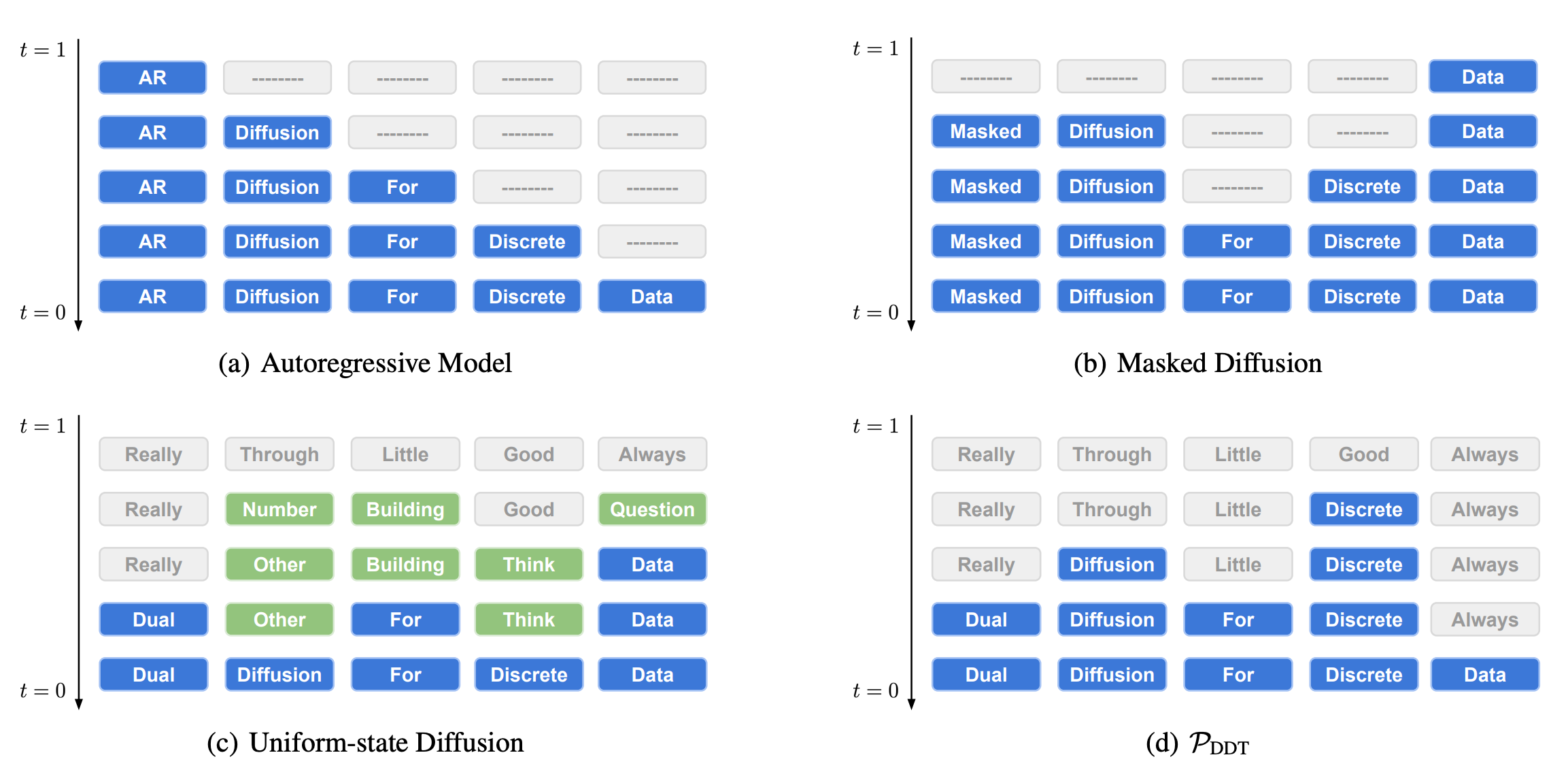
The inference loop of Uniform Diffusion is most easily understood by looking at the figure above from the Diffusion Duality paper. Auto-regressive modeling generates each token one at a time from left to right. Masked diffusion generates each token one at a time (of course, it is possible for masked diffusion to generate multiple tokens at once) in any order. However, masked diffusion shares the limiting characteristic of auto-regressive modeling that once you generate a token, that token cannot change. This limits its ability to do self-correction. In uniform-state diffusion, multiple tokens are generated at once, but generated tokens can still change during the diffusion process, allowing for self-correction. We will ignore the bottom-right sub-figure for this post.
Diffusion Preliminaries
Before we formulate how we would build a uniform-state diffusion model, let us review some preliminaries from diffusion (here is a past blog post with additional motivating details). Loosely speaking, diffusion can be thought of as interpolating between two distributions—a starting data distribution p_0 and a final prior distribution π that is easy to sample from (e.g. a Gaussian distribution for continuous data, a distribution of all mask tokens for masked diffusion, a uniform random distribution for uniform dstate diffusion). The diffusion process follows a diffusion schedule where at time t between 0 and 1, the data is interpolated a certain amount between p_0 and π.
The forward diffusion process transforms a point from data distribution to the prior distribution; this is easy as you simply corrupt the data. The reverse diffusion process, which is what we are trying to learn, transforms a point sampled from the prior distribution into the data distribution. Roughly speaking, the model is trained to make the reverse diffusion process approximate the inverse of the forward diffusion process by minimizing the negative ELBO loss.
Forward Diffusion for Uniform State Diffusion
As stated earlier, given a data point x, modeling the forward diffusion process q(z_t|x) is easy—you simply take x and interpolate it with the prior distribution. In continuous diffusion, x is an n-dimensional vector and you corrupt it by adding random Gaussian noise.
In uniform discrete diffusion, x is an n-dimensional one-hot vector that corresponds to a discrete variable that can take on one of n values (i.e. your vocab size for text diffusion). π is a uniform distribution where all n vocab words can be sampled with equal probability. The corruption process is thus given by:
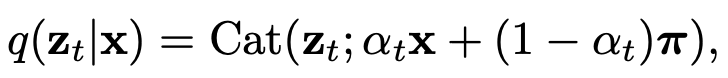
where α_t is a scheduler for how corrupted the data should be. In summary, at time t=1, z_t is a completely uniform distribution, at time t=0, z_t is the one-hot vector corresponding to the correct token, and for t between 0 and 1, z_t is a categorical distribution that lies somewhere in between these two extremes.
In continuous diffusion, the corruption process can be interpreted that at any given point in time, we are adding increasingly strong random Gaussian noise to our data point. In uniform state diffusion, the corruption process can be interpreted as that at any given point in time, with increasingly strong probability we will transition a token’s value to a uniformly random value.
Reverse Diffusion for Discrete Diffusion
The reverse diffusion process is a neural network that is trained to undo the corruption from the forward diffusion process. If you expand out the math for q(z_t|x) and follow the negative ELBO loss of the diffusion model (details are explained in Section 4 of Schiff et al ) and make the time-steps infinitesimally small, you get the final loss:

Here is a summary of how to interpret the loss. At each time-step t, we will corrupt x into x̄ and then sample a one-hot vector z_t from the normalized version of x̄. We then pass z_t into our neural network to get our reconstruction x̄_θ .The loss is the KL divergence between the ground truth corrupted distribution x̄ and the predicted corrupted distribution x̄_θ for every token in the sequence (hence the summation over l). i is the element of z_t that is non-zero (i.e. i is the sampled vocab word). This loss is summed over the entire sequence length l.
We see that when x̄_θ is exactly x̄, then the loss is 0 as expected. The first two terms within the bracket (N * [1/x̄_i - 1/x̄_θ_i]) will be positive if the reconstruction did not put enough probability density on element i. That is, that means the sampled token was actually correct, but the model mistakenly tried to self-correct and change that token.
Let us now look at the inner summation term on the right (apologies for Substack being awful for Latex). The term outside the log is a weighting term that essentially says, “weight this term heavier if the ground truth distribution should have actually put more density onto vocab word j compared to i.” The term within the log penalizes the model heaviest if it tried to self-correct, but it self-corrected to the wrong vocab word. It then obviously penalizes the model in the denominator if it did not put enough density onto the correct vocab word.
The loss is a bit dense, but in summary, roughly speaking the best thing the model can do is obviously to self-correct itself to the correct ground truth vocab word or not self-correct if the input is already correct. The next best thing to do is to not self-correct. Next is to self correct from something wrong onto something else wrong. The most heavily penalized behavior is to self-correct from something right onto something wrong.
Can Uniform State Diffusion Catch Up with Masked Diffusion?
As mentioned earlier, despite what I consider their aesthetic superiority, Schiff et al showed that uniform state diffusion still performs empirically worse than masked diffusion except in data with small vocab sizes such as DNA (the follow up Duo worked also showed that uniform state diffusion was superior in low inference-time compute situations, but we won’t discuss that here). Here is my hand-wavy intuition for why this is the case.
As I mentioned in my post on why I’m skeptical of masked diffusion, from an information theoretic perspective, masked diffusion seems to be less efficient than auto-regressive modeling. If I were to communicate the results of an auto-regressive model to you, I would only need to send over the bits corresponding to what vocab words I sampled in left-to-right order. However, for masked diffusion I need to additionally send over bits to describe the order in which my unmasking occured. This seems like extra overhead without any clear benefit.
For uniform state diffusion modeling, the overhead cost is even worse than masked diffusion. In masked diffusion, you only need to send over whether or not a masked token is going to be unmasked at that iteration. In uniform state diffusion modeling, you need to send over whether a token is being self-corrected for every token in your sequence, not just for the masked tokens. However, the elusive potential redeeming attribute of uniform state diffusion is that the ability to self-correct is helpful enough to override the extra overhead you’re paying to indicate which tokens need to be self-corrected. Hence, I would expect that more powerful models in the future with more capable self-correction would more heavily favor uniform state diffusion.
Why do lower vocab settings favor uniform state diffusion modeling? Imagine a toy setting where the model finds that every token could only take on one of two values with equal probability. Then, in masked diffusion, you have to spend bits to communicate over which tokens you are going to unmask as well as one bit for every unmasked token to communicate the value of that token. On the other hand, for uniform state diffusion, if you communicate that you are going to self-correct a token, then you don’t need to communicate the value you are self-correcting to; you can simply assume it is the other possible value. Thus, the lower vocab size is, the more it favors uniform state diffusion, because every time you communicate that you are self-correcting, you are removing the existing token from the pool of possible values that the token could possibly take on, thereby reducing the cost it sends to communicate the value of the correct token.
One of the core tenets of where I work is that tokenization sucks. One of tokenization’s many sins is that it blows up the vocabulary size, and it will be interesting to see if the end of tokenization brings about the rise of uniform state text diffusion.