
An Intuitive Intro to Flow Matching with Minimal Math
An intuition (and some math) of what is going on in a flow matching/diffusion model.

Flow matching is a powerful generative modeling framework that can be thought of as a generalization of diffusion. The zero-math summary of diffusion/flow matching is we train a model by adding noise to a ton of training examples and learning to denoise the examples; we can then sample pretty images by running this denoiser many times.
Unfortunately, any sort of deeper intuitive understanding of diffusion and flow matching requires some math, but once you get over the hump it really is quite beautiful. This post intends to gently ease our way into the math in order to provide a solid intuitive understanding of flow matching for anyone with a CS background.
This post is based off of Section 2 from Meta’s Flow Matching Guide and Code. All figures and code are from the guide unless stated otherwise.
Diffusion Modeling Problem Statement
All data (e.g. the manifold of natural images) lies on a distribution q. We would like to sample on q, but it is complex and intractable to directly sample from. Instead, we will sample from a Gaussian noise distribution p (which is easy to sample from) and then simply learn the transformation from p to q using a neural network (i.e. our diffusion/flow-matching model).
Diffusion and flow-matching models leverage the neural network to model this transformation by using differential equations. Differential equations may seem scary and abstract, but we only seek a high level intuition and motivation, making our lives easier.
Differential Equations Intuition
What are differential equations? Why do we care about them? Why are they so important to the diffusion literature? Imagine you’re a tiny ant on a smooth surface.
You have no global information of where you are on this surface. However, you can observe the surface around you to understand local information like the gradient of the surface. Now, suppose I drop you off on the surface and tell you what your initial position is. You start walking. You can figure out where you are in space at any time by taking your initial position and integrating (i.e. take a bunch of sums) the local gradient information you observe at every step.
This sets up the differential equations we learned in freshman year of college, which in the one-dimensional case looks something like this.
We have a function y(t). We can easily measure the local change of y based on the values of y and t (e.g. we can guess how fast the rabbit population will increase based on the season and how many rabbits there are). If we also know y(0) (e.g. how many rabbits there were when we started), then we can solve for the value of y(t) (e.g. the rabbit population) at any time t.
One example of how to solve a differential equation is Euler’s Method, which is what most people would intuitively come up with. Starting from y_0, you take a bunch of small steps of size h and follow the gradient at each time-step. Formally, this looks like:
Of course, more complicated and higher-order methods exist, but we don’t need to go into that. For the purposes of this post, just remember:
Differential equations arise when we easily know the gradient of a function rather than the value of the function itself.
We can solve differential equations to model the value of the function everywhere in input space by stepping along the function gradient.
Diffusion-Differential Equation Analogy
Let’s come up with a rough visual intuition for diffusion now. We will get into more specifics later. Roughly speaking, diffusion/flow-matching transforms a simple noise distribution p into the data complex distribution q. We can think of p(x) as an initial distribution across out input space at time t=0, and q(x) as our final target distribution at time t=1. There is some continuous transformation function along time that maps from p to q. However, directly modeling the transformation from p to q feels intractable. Remember you’re not just transforming two points. You’re transforming two entire distributions; you need global knowledge of how your entire data is distributed (e.g. the manifold of all images).
However, we can still sample from q without a global understanding of the distribution. First, we sample a specific point from p. This can be thought of like dropping off our ant on a specific point in the space-time manifold. Now, our tiny ant can travel across time by stepping along the gradient of the data manifold—which is easier to estimate because it is a local attribute of what the distribution looks like at that specific data point—until it reaches a point in q at t=1. What a diffusion/flow-matching model essentially does is estimate this gradient. Given a point x and a time-step t, the neural network predicts the gradient of our manifold of distributions, which we follow along to push a point from our noise distribution to the data distribution, thereby generating a sample.
As an aside, another popular machine learning paradigm that uses a neural network to predict local information and then integrates along local information to get a global picture is the Neural Radiance Field (NeRF) stream of work for representing a 3D scene.
Understanding the Flow Matching Objective
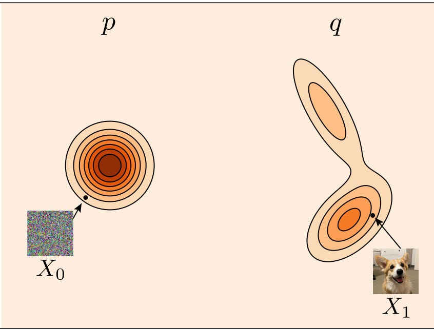
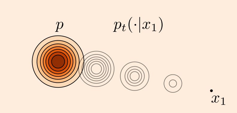
Let’s get into the specifics of flow matching. Here is a visualization of what p and q look like. p is a Gaussian noise distribution that is easy to sample from. q is our final complicated data distribution. For those unfamiliar with these types of figures, a darker color indicates higher probability density and a lighter color indicates lower probability density.
Now, we can visualize what does it mean to transform p into q. We define a family of distributions p_t where p_0=p and p_1=q. We define p_t at any time t between 0 and 1 to be the linear interpolation between p and q.
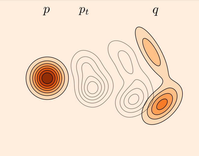
Algebraically, the definition of p_t looks something like:
These equations are saying that if we sample a random variable X_0 from p and a random variable X_1 from q, the random variable X_t from the distribution p_t is the linear interpolation between X_0 and X_1.
Now we just need to train a neural network to model this transformation of p along time. At any time t, we are interested in finding the velocity field u_t(x), which is the direction that points from p_t to q at any point x. The flow matching objective of neural network parameters θ thus looks something like:
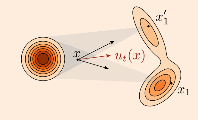
The flow matching objective minimizes the expectation—across all time values t and all members X_t of the distribution p_t—of the L2 error of the predicted velocity field and the true velocity field. Geometrically, we can think of the velocity field as the direction we would push each point in the distribution p_t to “warp” it so that it looks like q. Visually, this looks something like:
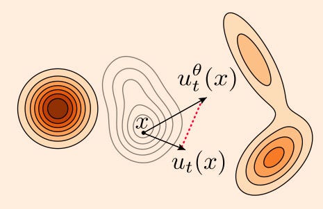
In order to warp p_t to q, we need to push it in the direction of u_t(x). We want to minimize the expected value—across all points in space-time—of the length of the red dotted line, which represents the error between the predicted velocity field and the ground truth velocity field.
However, we don’t know the ground truth value u_t(x). In this toy example, we can kind of see what u_t(x) should look like because it’s low dimensional and we know what q looks like, but recall that in practice, if q is something complex and high-dimensional like the distribution of all natural images, we don’t know what q looks like. How are we going to estimate the correct transformation when we don’t even know what the target distribution looks like?
But all is not lost. We can simplify the objective by conditioning on a specific data point x_1 from q (i.e. by sampling an example from our training set). Now if we linearly interpolate between p and x_1, all our intermediate distributions p_t are nice Gaussians with decreasing variance.
u_t(x|x_1) is really easy to calculate now: it simply points in the direction from x to x_1. Algebraically, this means that if we have,
then the value of the velocity field at x is simply given by x_1-x_0.
We can now perform marginalization, which means we will estimate the true value of u_t(x) by taking the expectation of all conditional probabilities over all possible conditions. In practice, this means that we will simply train on our entire training set and try to minimize the expected value of the objective. In the figure below, we see that the velocity field can point in two very different directions if we condition on two different points from q, but we can arrive at an estimate of the true direction by taking the mean.
Putting this all together, we can write down the flow matching objective as:
To estimate this expectation, you simply sample a timestep t, a training example x_1, and a noise vector x_0 and generate the appropriate x_t and then calculate the mean squared error of the estimated the velocity field over all your samples.
In Pytorch, the training loop is as simple as:
for _ in range(10000):
x_1 = sample_data()
x_0 = torch.randn_like(x_1)
t = torch.rand(len(x_1), 1)
x_t = (1 - t) * x_0 + t * x_1
dx_t = x_1 - x_0
optimizer.zero_grad()
F.mse(flow(x_t, t), dx_t).backward()
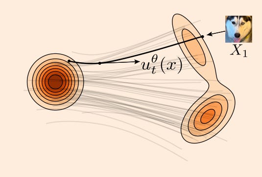
optimizer.step()To sample from the model, you simply randomly sample noise and then use your favorite ODE-solver to integrate along the velocity fields by using your model to estimate the velocity field at each step of the solver. Geometrically, this looks something like:
You can take a look at the full training and sampling example from section 2 of Meta’s tutorial.
Relationship with Diffusion
Those familiar with diffusion will notice that the flow matching is basically the same as diffusion: corrupt data with Gaussian noise, train a neural network to recover the original data, plug the neural network into some differential equation solver to sample from the data distribution. In fact, a recent blog from Google Deepmind shows that there is no fundamental difference between Gaussian flow matching (i.e. when the source distribution p is a Gaussian) and diffusion. Thus, flow matching can be thought of as a generalization of diffusion.
Why should we care about flow matching if it’s just another interpretation of diffusion? Aside from alternative interpretations making things feel more beautiful and fundamental, there are two practical reasons to care about diffusion.
The alternative flow-matching interpretation can yield insights on how to improve practical problems in diffusion like reducing the number of steps needed for each sample and being more amenable to RL;HF fine-tuning.
Gaussian noise corruption seems to be awesome for images and maybe audio. However, there may be cases where we don’t want a Gaussian source distribution or we don’t want interpolation to be done in Euclidean space. The more general flow-matching paradigm can thus be extended to arbitrary data modalities, including discrete modalities like text.