
Three Interpretations of DeepSeek V2's Multi-headed Latent Attention Layer
UnderstandingWhy MLA's Results Are So Good

DeepSeek V2’s key contribution to improve computational efficiency is Multi-headed Latent Attention (MLA), which is both faster and stronger compared to all previous attention variants. In this post, I go over three different interpretations of MLA:
A Natural Generalization of Group Query Attention (GQA).
A More Efficient Version of Multi Query Attention (MQA) in Higher Dimensions.
Multi-Headed Attention (MHA) with An Inductive Bias for Low Dimensionality.
The first interpretation is pretty much a wrapper around the definition of MLA. I think it’s pretty much correct in that there are no incorrect statements, but it doesn’t do a great job explaining why MLA is even better than MHA, which I found to be a surprising result.
I present two alternative interpretations that are plausible but not necessarily correct. However, they would more comprehensively explain MLA’s results.
I skip over most of MLA’s technical details as they are quite straightforward and can be found in the DeepSeek V2 paper or various other blog posts. Readers are also encouraged to read some blogs about attention and KV caching for better context, but I tried to keep this post self-contained.
Background
Attention
What we do in attention is that we construct a key-value pair for each token in our input. The key indicates what type of information each token provides, and the value indicates what the information actually is. We then query the set of key-value pairs by creating a query vector and taking its dot product with every single key. We then update our representation with the values of the <key, value> pairs that had high dot product similarity with the query. What makes attention powerful is that no matter how large and complicated the input is (e.g. a really long piece of text), attention can pick out the relevant inputs while ignoring everything else.
For example, suppose we are trying to build a representation of a man’s dating profile. We receive the description, “a man in finance, 6’ 5”, trust fund, blue eyes.” The key-value papers that might be generated would be <career, finance>, <height, 6’ 5”>, <wealth, trust fund>, <eye color, blue>. We can then submit a query such as “eye color”. The query will have a low similarity score with all the keys other than “eye color”, so the attention layer will learn to focus its attention on <eye color, blue> while ignoring the rest of the inputs, and update the representation so that it knows that the man has blue eyes.
A key-value cache caches the attention layer’s key-value pairs during model inference to improve speed. The only relevant aspect of the key-value cache to our discussion is we want to reduce the size of the cache to improve efficiency by reducing the number of key-value pairs we need to cache. MLA’s key contribution is reducing this number.
Multi-Headed Attention
We are typically interested in multiple attributes and would like to make multiple different queries. In our example, we are probably also interested in adding the man’s wealth, career, and height into our representation. We would thus also want to run queries on all these other attributes. Multi-Headed Attention (MHA) parallelizes this process by running multiple copies of attention (each copy is called a head) at once and then concatenating the results together. This is more effective than running one giant attention head on a single high-dimensional query-key-value space, since each head can learn to attend to different tokens in the input, creating a very rich representation.
Multi-Query Attention
In our toy example, the queries across different heads will be extremely diverse as they are all querying different attributes (e.g. “eye color” vs “height”). However, we could likely get away with using the same key-value pairs across all heads as they simply describe the attribute and attribute type of each token, which remains the same across different heads (e.g. <eye color, blue> is a decent key-value pair across all different heads). Multi-Query Attention (MQA) is thus a natural follow-up to MHA that shares the key-value pairs across all heads, which significantly reduces the compute while leading to a small but noticeable degradation in performance.
Group-Query Attention
Let us now take a look at a visualization between MHA and MQA in a figure from DeepSeekV2. A bar with stripes corresponds to an item that needs to be stored in the KV cache. We see that MQA has one shared key-value pair for all heads, and MHA has a key-value pair for every head. MHA clearly requires more computation than MQA, but performs better as well.
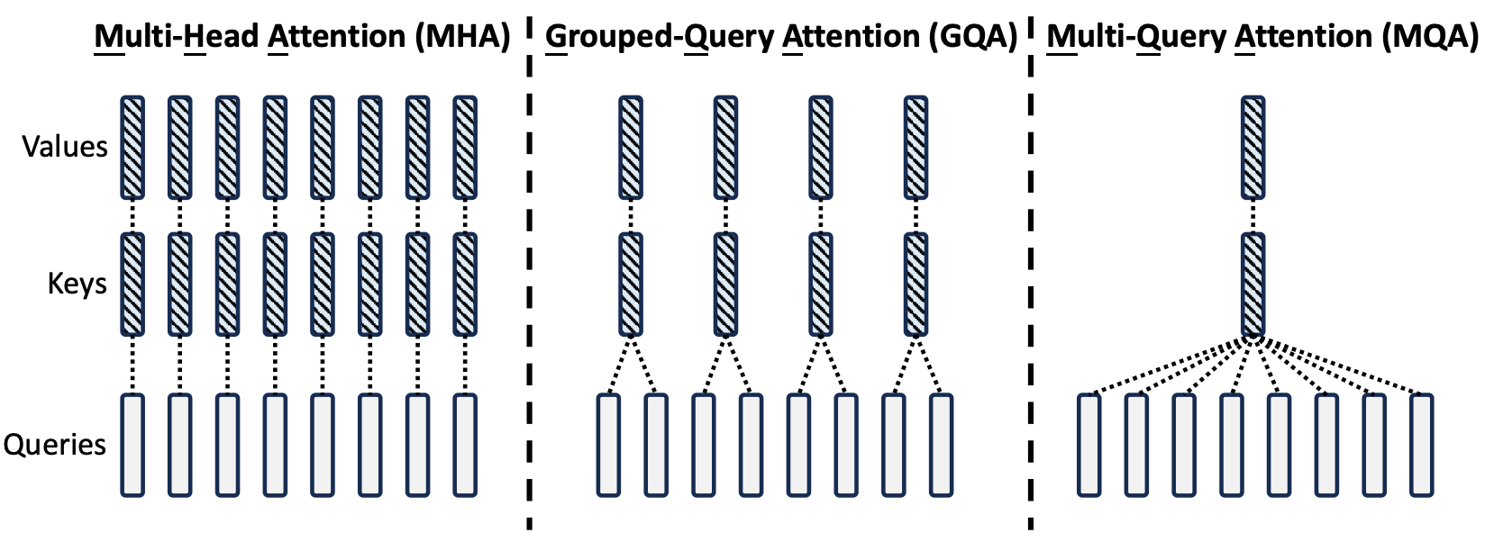
GQA is yet another obvious follow-up that interpolates along the efficiency-quality trade-off between MHA and MQA by sharing key-value pairs between some heads but not all—heads are grouped together, and key-value pairs are shared between heads within the same group.
Multi-head Latent Attention
Interpretation #1: A Natural Generalization of GQA
Consider the visualization of GQA above. Suppose we concatenated the four key-value pairs together to form one big latent representation of the key-value pairs. We can then down-project from the latent representation to create a unique key-value pair for each head. Only the latent representation needs to be stored in the KV cache, as seen in the figure below.
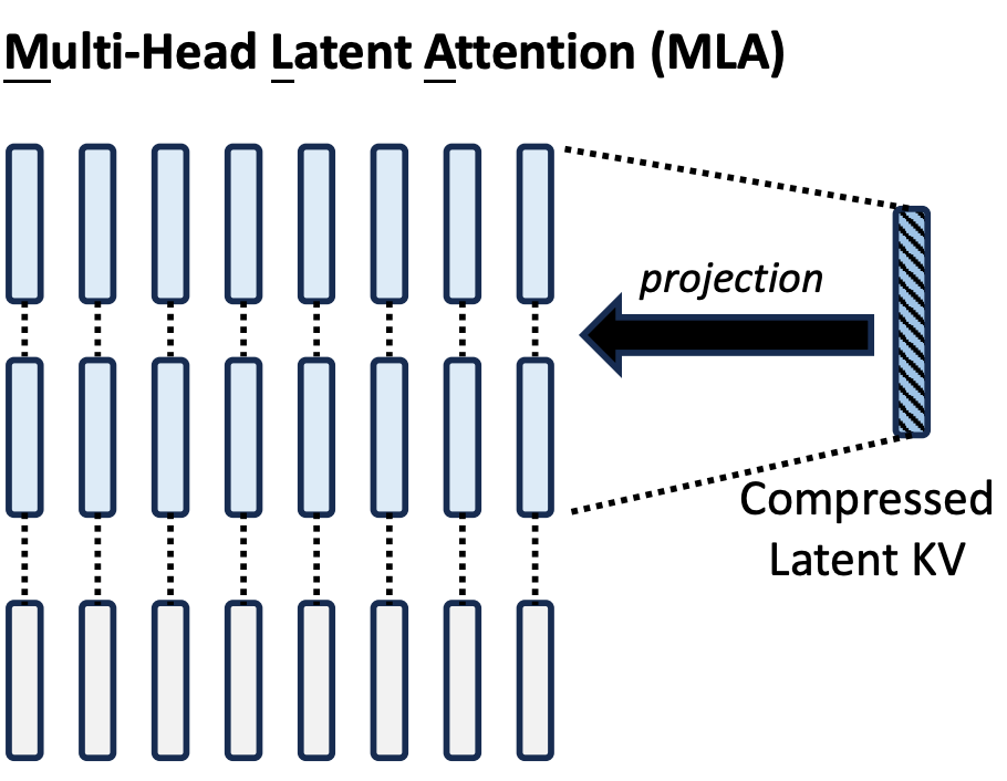
We can learn the projection matrix to exactly recover GQA (i.e. each row in the projection matrix corresponds to a dimension of the latent vector, with a 1 in the column corresponding to the group it belongs to and 0 everywhere else), so in this sense MLA can be viewed as a strictly better and more general version of GQA and therefore a natural follow-up.
This interpretation appears to be true as it is practically a wrapper around the definition, but I don’t think it’s particularly interesting.
Interpretation #2: A More Efficient Version of Higher-Dimensional MQA
The powerful aspect of attention is that you can attend to the relevant token while ignoring all the other irrelevant tokens. In order for that to happen well on MQA, you roughly need the keys of all the tokens to be orthogonal. For example, if I query for “eye color,” but there is also a “hair color” key that is close to “eye color” in embedding space, then my results will sum the values of “eye color” and “hair color,” and the model will assume conclude that the man’s eye color is some combination of blue and blonde.
If my embedding space of keys is too tight to make key concepts orthogonal to each other, one solution is to expand the dimensionality of embedding space. Of course, the problem is that this is more expensive.
One interpretation of MLA is that it is a more efficient version of a higher dimensional MQA. In high-dimensional space, hair color, eye color, occupation, and height would all be orthogonal vectors from each other. However, if one of our heads is making queries related to colors, we don’t need occupation and height to be orthogonal to each other; they can all just map to the same null vector instead. Hence, it is safe to down-project our high-dimensional vector to a lower-dimensional vector and discard information that is irrelevant to our query. MLA can thus possibly be interpreted as MQA at the dimensionality of the latent vector but at the computational cost of the dimensionality of the key vectors.
Interpretation #1 explains why MLA is better than MQA and GQA at equivalent group counts, but why does MLA somehow perform better than MHA at the same level of dimensionality? After all, going purely by expressive capacity, MHA is strictly better than MLA. MLA must provide some sort of inductive bias that MHA does not.
Under Interpretation #2, MLA is guiding the model to act like a higher dimensional, more powerful attention model. Even though a standard MHA is in principle capable of representing this structure of a high-dimensional vector projected onto many heads, it might not be able to figure this structure out by itself during the optimization process. The structured guidance would thus give MLA its superior performance over MHA.
Interpretation #3: MHA with an Inductive Bias for Low Dimensionality
Interpretation #2 compares the dimensionality of the latent with the dimensionality of the individual keys and values, so it suggests MLA is powerful because it provides an inductive bias to act like a high-dimensional model. On the other hand, when compared to the combined dimensionality of all the heads, MLA can alternatively be viewed as providing an inductive bias to behave like a low-dimensional model.
Suppose I wanted to represent 1000 different classes of animals in an embedding space. I can represent each animal as a one-hot 1000-dimensional vector, with each dimension corresponding to a different animal. This is a highly expressive representation, but it is not particularly useful. If I give you such an embedding of an animal, all you will know is its name.
However, if I force every animal into a lower dimensional space, it is impossible to make every single animal’s embedding orthogonal to each other. The embedding space thus has to make some concessions and make certain animals point in similar directions in embedding space. If you learn a low-dimensional embedding space in any sort of normal machine learning framework, the embedding space will naturally learn to put similar animals (e.g. tigers and lions) closer together and make truly unrelated animals (e.g. tigers and fish) completely orthogonal to each other.
Now, if I hand you such an embedding for an animal you are unfamiliar with, by observing where it is in embedding space and who its neighbors are, you will be able to figure out a lot about the animal. Even though the low-capacity representation is less expressive, it is arguably more intelligent than the higher dimensional representation. Using low-capacity representations to improve generalization and transfer learning capabilities is thus a common practice in machine learning. This can be summarized as Occam’s Razor, which says that the simplest, least complex model is best at explaining the evidence.
It is possible something like this is happening in MLA as well. There is clearly a lot of redundancy among the key-value pairs in MHA; otherwise MQA would not work so well. Perhaps what MLA does is compress these redundancies into a lower dimensional representation, which forces the model to learn relationships and similarities between different heads. By forcing the model to explicitly reason about the relationship between heads, perhaps it learns fundamental underlying structures that generalize well to new tasks or is forced to eliminate redundancies among the heads in order to best utilize the low-dimensional latent space.
Conclusion
MLA is not the first deep learning solution that works surprisingly effectively for reasons that are not 100% clear. Based on my views of deep learning’s trend towards over-parameterization and increasing expressive power and letting the model figure everything out, I would lean towards Interpretation #2 as the correct interpretation for why MLA is so powerful. However, Interpretation #3 would make some sense to me too even though it is kind of the opposite. Empirically, the correctness of Interpretation #2 would be easy to test by comparing MLA to a higher-dimensional MQA model (which would have more parameters). My prediction would be that they perform similarly, but I wouldn’t be surprised to be wrong.